
A Simple Approach to Linear Regression
Media company case study approach - solving a real problem using Linear regression

Linear regression is the next step up after correlation. It is used when we want to predict the value of a variable based on the value of another variable. The variable we want to predict is called the dependent variable (or sometimes, the outcome variable)

However, for new data scientists, it could get overwhelming. Hence in this blog I have shared an iterative approach and perhaps is how we do it in large companies as well.
It is assumed that the reader can follow the code, all the conceptual explanations are omitted intentionally to keep the focus on the code. Code is adequately documented. It is also understood that the reader is a beginner in data science however knows statistics and python.
Also published on - https://maddymaster.medium.com/media-company-case-study-1a06334f672d
Lets begin:
Media Company Case Study
Problem Statement: A digital media company (similar to Voot, Hotstar, Netflix, etc.) had launched a show. Initially, the show got a good response, but then witnessed a decline in viewership. The company wants to figure out what went wrong.
In [317]:
# Importing all required packagesimportnumpyasnpimportpandasaspdimportmatplotlib.pyplotaspltimportseabornassns%matplotlib inlineIn [318]:
#Importing datasetmedia = pd.read_csv('mediacompany.csv')media = media.drop('Unnamed: 7',axis = 1)In [319]:
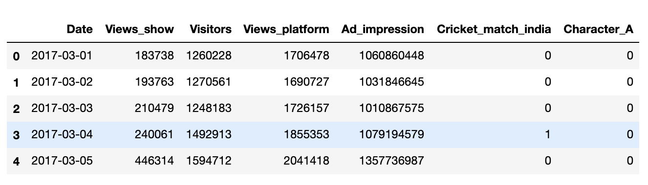
#Let's explore the top 5 rowsmedia.head()Out[319]:

In [320]:
# Converting date to Pandas datetime formatmedia['Date'] = pd.to_datetime(media['Date'])In [321]:
media.head()Out[321]:
In [322]:
# Deriving "days since the show started"fromdatetimeimport dated0 = date(2017, 2, 28)d1 = media.Datedelta = d1 - d0media['day']= deltaIn [323]:
media.head()Out[323]:

In [324]:
# Cleaning daysmedia['day'] = media['day'].astype(str)media['day'] = media['day'].map(lambda x: x[0:2])media['day'] = media['day'].astype(int)In [325]:
media.head()Out[325]:

In [326]:
# days vs Views_showmedia.plot.line(x='day', y='Views_show')Out[326]:

In [327]:
# Scatter Plot (days vs Views_show)colors = (0,0,0)area = np.pi*3plt.scatter(media.day, media.Views_show, s=area, c=colors, alpha=0.5)plt.title('Scatter plot pythonspot.com')plt.xlabel('x')plt.ylabel('y')plt.show()
In [328]:
# plot for days vs Views_show and days vs Ad_impressionsfig = plt.figure()host = fig.add_subplot(111)par1 = host.twinx()par2 = host.twinx()host.set_xlabel("Day")host.set_ylabel("View_Show")par1.set_ylabel("Ad_impression")color1 = plt.cm.viridis(0)color2 = plt.cm.viridis(0.5)color3 = plt.cm.viridis(.9)p1, = host.plot(media.day,media.Views_show, color=color1,label="View_Show")p2, = par1.plot(media.day,media.Ad_impression,color=color2, label="Ad_impression")lns = [p1, p2]host.legend(handles=lns, loc='best')# right, left, top, bottompar2.spines['right'].set_position(('outward', 60)) # no x-ticks par2.xaxis.set_ticks([])# Sometimes handy, same for xaxis#par2.yaxis.set_ticks_position('right')host.yaxis.label.set_color(p1.get_color())par1.yaxis.label.set_color(p2.get_color())plt.savefig("pyplot_multiple_y-axis.png", bbox_inches='tight')
In [329]:
# Derived Metrics# Weekdays are taken such that 1 corresponds to Sunday and 7 to Saturday# Generate the weekday variablemedia['weekday'] = (media['day']+3)%7media.weekday.replace(0,7, inplace=True)media['weekday'] = media['weekday'].astype(int)media.head()Out[329]:

Running first model (lm1) Weekday & visitors
In [330]:
# Putting feature variable to XX = media[['Visitors','weekday']]# Putting response variable to yy = media['Views_show']In [331]:
fromsklearn.linear_modelimport LinearRegressionIn [332]:
# Representing LinearRegression as lr(Creating LinearRegression Object)lm = LinearRegression()In [333]:
# fit the model to the training datalm.fit(X,y)Out[333]:
LinearRegression(copy_X=True, fit_intercept=True, n_jobs=1, normalize=False)In [334]:
importstatsmodels.apiassm#Unlike SKLearn, statsmodels don't automatically fit a constant, #so you need to use the method sm.add_constant(X) in order to add a constant. X = sm.add_constant(X)# create a fitted model in one linelm_1 = sm.OLS(y,X).fit()print(lm_1.summary())OLS Regression Results ==============================================================================Dep. Variable: Views_show R-squared: 0.485Model: OLS Adj. R-squared: 0.472Method: Least Squares F-statistic: 36.26Date: Fri, 09 Mar 2018 Prob (F-statistic): 8.01e-12Time: 10:27:35 Log-Likelihood: -1042.5No. Observations: 80 AIC: 2091.Df Residuals: 77 BIC: 2098.Df Model: 2 Covariance Type: nonrobust ============================================================================== coef std err t P>|t| [0.025 0.975]------------------------------------------------------------------------------const -3.862e+04 1.07e+05 -0.360 0.720 -2.52e+05 1.75e+05Visitors 0.2787 0.057 4.911 0.000 0.166 0.392weekday -3.591e+04 6591.205 -5.448 0.000 -4.9e+04 -2.28e+04==============================================================================Omnibus: 2.684 Durbin-Watson: 0.650Prob(Omnibus): 0.261 Jarque-Bera (JB): 2.653Skew: 0.423 Prob(JB): 0.265Kurtosis: 2.718 Cond. No. 1.46e+07==============================================================================Warnings:[1] Standard Errors assume that the covariance matrix of the errors is correctly specified.[2] The condition number is large, 1.46e+07. This might indicate that there arestrong multicollinearity or other numerical problems.In [335]:
# create Weekend variable, with value 1 at weekends and 0 at weekdaysdef cond(i): if i % 7 == 5: return 1 elif i % 7 == 4: return 1 else :return 0 return imedia['weekend']=[cond(i) for i in media['day']]In [336]:
media.head()Out[336]:

Running second model (lm2) visitors & weekend
In [337]:
# Putting feature variable to XX = media[['Visitors','weekend']]# Putting response variable to yy = media['Views_show']In [338]:
importstatsmodels.apiassm#Unlike SKLearn, statsmodels don't automatically fit a constant, #so you need to use the method sm.add_constant(X) in order to add a constant. X = sm.add_constant(X)# create a fitted model in one linelm_2 = sm.OLS(y,X).fit()print(lm_2.summary())OLS Regression Results ==============================================================================Dep. Variable: Views_show R-squared: 0.500Model: OLS Adj. R-squared: 0.487Method: Least Squares F-statistic: 38.55Date: Fri, 09 Mar 2018 Prob (F-statistic): 2.51e-12Time: 10:27:35 Log-Likelihood: -1041.3No. Observations: 80 AIC: 2089.Df Residuals: 77 BIC: 2096.Df Model: 2 Covariance Type: nonrobust ============================================================================== coef std err t P>|t| [0.025 0.975]------------------------------------------------------------------------------const -8.833e+04 1.01e+05 -0.875 0.384 -2.89e+05 1.13e+05Visitors 0.1934 0.061 3.160 0.002 0.071 0.315weekend 1.807e+05 3.15e+04 5.740 0.000 1.18e+05 2.43e+05==============================================================================Omnibus: 1.302 Durbin-Watson: 1.254Prob(Omnibus): 0.521 Jarque-Bera (JB): 1.367Skew: 0.270 Prob(JB): 0.505Kurtosis: 2.656 Cond. No. 1.41e+07==============================================================================Warnings:[1] Standard Errors assume that the covariance matrix of the errors is correctly specified.[2] The condition number is large, 1.41e+07. This might indicate that there arestrong multicollinearity or other numerical problems.Running third model (lm3) visitors, weekend & Character_A
In [339]:
# Putting feature variable to XX = media[['Visitors','weekend','Character_A']]# Putting response variable to yy = media['Views_show']In [340]:
importstatsmodels.apiassm#Unlike SKLearn, statsmodels don't automatically fit a constant, #so you need to use the method sm.add_constant(X) in order to add a constant. X = sm.add_constant(X)# create a fitted model in one linelm_3 = sm.OLS(y,X).fit()print(lm_3.summary())OLS Regression Results ==============================================================================Dep. Variable: Views_show R-squared: 0.586Model: OLS Adj. R-squared: 0.570Method: Least Squares F-statistic: 35.84Date: Fri, 09 Mar 2018 Prob (F-statistic): 1.53e-14Time: 10:27:35 Log-Likelihood: -1033.8No. Observations: 80 AIC: 2076.Df Residuals: 76 BIC: 2085.Df Model: 3 Covariance Type: nonrobust =============================================================================== coef std err t P>|t| [0.025 0.975]-------------------------------------------------------------------------------const -4.722e+04 9.31e+04 -0.507 0.613 -2.33e+05 1.38e+05Visitors 0.1480 0.057 2.586 0.012 0.034 0.262weekend 1.812e+05 2.89e+04 6.281 0.000 1.24e+05 2.39e+05Character_A 9.542e+04 2.41e+04 3.963 0.000 4.75e+04 1.43e+05==============================================================================Omnibus: 0.908 Durbin-Watson: 1.600Prob(Omnibus): 0.635 Jarque-Bera (JB): 0.876Skew: -0.009 Prob(JB): 0.645Kurtosis: 2.488 Cond. No. 1.42e+07==============================================================================Warnings:[1] Standard Errors assume that the covariance matrix of the errors is correctly specified.[2] The condition number is large, 1.42e+07. This might indicate that there arestrong multicollinearity or other numerical problems.In [341]:
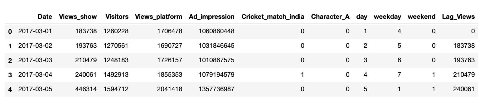
# Create lag variablemedia['Lag_Views'] = np.roll(media['Views_show'], 1)media.Lag_Views.replace(108961,0, inplace=True)In [342]:
media.head()Out[342]:
Running fourth model (lm4) visitors, Character_A, Lag_views & weekend
In [343]:
# Putting feature variable to XX = media[['Visitors','Character_A','Lag_Views','weekend']]# Putting response variable to yy = media['Views_show']In [344]:
importstatsmodels.apiassm#Unlike SKLearn, statsmodels don't automatically fit a constant, #so you need to use the method sm.add_constant(X) in order to add a constant. X = sm.add_constant(X)# create a fitted model in one linelm_4 = sm.OLS(y,X).fit()print(lm_4.summary())OLS Regression Results ==============================================================================Dep. Variable: Views_show R-squared: 0.740Model: OLS Adj. R-squared: 0.726Method: Least Squares F-statistic: 53.46Date: Fri, 09 Mar 2018 Prob (F-statistic): 3.16e-21Time: 10:27:36 Log-Likelihood: -1015.1No. Observations: 80 AIC: 2040.Df Residuals: 75 BIC: 2052.Df Model: 4 Covariance Type: nonrobust =============================================================================== coef std err t P>|t| [0.025 0.975]-------------------------------------------------------------------------------const -2.98e+04 7.43e+04 -0.401 0.689 -1.78e+05 1.18e+05Visitors 0.0659 0.047 1.394 0.167 -0.028 0.160Character_A 5.527e+04 2.01e+04 2.748 0.008 1.52e+04 9.53e+04Lag_Views 0.4317 0.065 6.679 0.000 0.303 0.560weekend 2.273e+05 2.4e+04 9.467 0.000 1.79e+05 2.75e+05==============================================================================Omnibus: 1.425 Durbin-Watson: 2.626Prob(Omnibus): 0.491 Jarque-Bera (JB): 0.821Skew: -0.130 Prob(JB): 0.663Kurtosis: 3.423 Cond. No. 1.44e+07==============================================================================Warnings:[1] Standard Errors assume that the covariance matrix of the errors is correctly specified.[2] The condition number is large, 1.44e+07. This might indicate that there arestrong multicollinearity or other numerical problems.In [345]:
plt.figure(figsize = (20,10)) # Size of the figuresns.heatmap(media.corr(),annot = True)
Out[345]:
<matplotlib.axes._subplots.AxesSubplot at 0x1d2cc0301d0>Running fifth model (lm5) Character_A, weekend & Views_platform
In [346]:
# Putting feature variable to XX = media[['weekend','Character_A','Views_platform']]# Putting response variable to yy = media['Views_show']In [347]:
importstatsmodels.apiassm#Unlike SKLearn, statsmodels don't automatically fit a constant, #so you need to use the method sm.add_constant(X) in order to add a constant. X = sm.add_constant(X)# create a fitted model in one linelm_5 = sm.OLS(y,X).fit()print(lm_5.summary())OLS Regression Results ==============================================================================Dep. Variable: Views_show R-squared: 0.602Model: OLS Adj. R-squared: 0.586Method: Least Squares F-statistic: 38.24Date: Fri, 09 Mar 2018 Prob (F-statistic): 3.59e-15Time: 10:27:37 Log-Likelihood: -1032.3No. Observations: 80 AIC: 2073.Df Residuals: 76 BIC: 2082.Df Model: 3 Covariance Type: nonrobust ================================================================================== coef std err t P>|t| [0.025 0.975]----------------------------------------------------------------------------------const -1.205e+05 9.97e+04 -1.208 0.231 -3.19e+05 7.81e+04weekend 1.781e+05 2.78e+04 6.410 0.000 1.23e+05 2.33e+05Character_A 7.062e+04 2.6e+04 2.717 0.008 1.89e+04 1.22e+05Views_platform 0.1507 0.048 3.152 0.002 0.055 0.246==============================================================================Omnibus: 4.279 Durbin-Watson: 1.516Prob(Omnibus): 0.118 Jarque-Bera (JB): 2.153Skew: 0.061 Prob(JB): 0.341Kurtosis: 2.206 Cond. No. 2.03e+07==============================================================================Warnings:[1] Standard Errors assume that the covariance matrix of the errors is correctly specified.[2] The condition number is large, 2.03e+07. This might indicate that there arestrong multicollinearity or other numerical problems.Running sixth model (lm6) Character_A, weekend & Visitors
In [348]:
# Putting feature variable to XX = media[['weekend','Character_A','Visitors']]# Putting response variable to yy = media['Views_show']In [349]:
importstatsmodels.apiassm#Unlike SKLearn, statsmodels don't automatically fit a constant, #so you need to use the method sm.add_constant(X) in order to add a constant. X = sm.add_constant(X)# create a fitted model in one linelm_6 = sm.OLS(y,X).fit()print(lm_6.summary())OLS Regression Results ==============================================================================Dep. Variable: Views_show R-squared: 0.586Model: OLS Adj. R-squared: 0.570Method: Least Squares F-statistic: 35.84Date: Fri, 09 Mar 2018 Prob (F-statistic): 1.53e-14Time: 10:27:37 Log-Likelihood: -1033.8No. Observations: 80 AIC: 2076.Df Residuals: 76 BIC: 2085.Df Model: 3 Covariance Type: nonrobust =============================================================================== coef std err t P>|t| [0.025 0.975]-------------------------------------------------------------------------------const -4.722e+04 9.31e+04 -0.507 0.613 -2.33e+05 1.38e+05weekend 1.812e+05 2.89e+04 6.281 0.000 1.24e+05 2.39e+05Character_A 9.542e+04 2.41e+04 3.963 0.000 4.75e+04 1.43e+05Visitors 0.1480 0.057 2.586 0.012 0.034 0.262==============================================================================Omnibus: 0.908 Durbin-Watson: 1.600Prob(Omnibus): 0.635 Jarque-Bera (JB): 0.876Skew: -0.009 Prob(JB): 0.645Kurtosis: 2.488 Cond. No. 1.42e+07==============================================================================Warnings:[1] Standard Errors assume that the covariance matrix of the errors is correctly specified.[2] The condition number is large, 1.42e+07. This might indicate that there arestrong multicollinearity or other numerical problems.Running seventh model (lm7) Character_A, weekend, Visitors & Ad_impressions
In [350]:
# Putting feature variable to XX = media[['weekend','Character_A','Visitors','Ad_impression']]# Putting response variable to yy = media['Views_show']In [351]:
importstatsmodels.apiassm#Unlike SKLearn, statsmodels don't automatically fit a constant, #so you need to use the method sm.add_constant(X) in order to add a constant. X = sm.add_constant(X)# create a fitted model in one linelm_7 = sm.OLS(y,X).fit()print(lm_7.summary())OLS Regression Results ==============================================================================Dep. Variable: Views_show R-squared: 0.803Model: OLS Adj. R-squared: 0.792Method: Least Squares F-statistic: 76.40Date: Fri, 09 Mar 2018 Prob (F-statistic): 1.10e-25Time: 10:27:38 Log-Likelihood: -1004.1No. Observations: 80 AIC: 2018.Df Residuals: 75 BIC: 2030.Df Model: 4 Covariance Type: nonrobust ================================================================================= coef std err t P>|t| [0.025 0.975]---------------------------------------------------------------------------------const -2.834e+05 6.97e+04 -4.067 0.000 -4.22e+05 -1.45e+05weekend 1.485e+05 2.04e+04 7.296 0.000 1.08e+05 1.89e+05Character_A -2.934e+04 2.16e+04 -1.356 0.179 -7.24e+04 1.38e+04Visitors 0.0144 0.042 0.340 0.735 -0.070 0.099Ad_impression 0.0004 3.96e-05 9.090 0.000 0.000 0.000==============================================================================Omnibus: 4.808 Durbin-Watson: 1.166Prob(Omnibus): 0.090 Jarque-Bera (JB): 4.007Skew: 0.476 Prob(JB): 0.135Kurtosis: 3.545 Cond. No. 1.32e+10==============================================================================Warnings:[1] Standard Errors assume that the covariance matrix of the errors is correctly specified.[2] The condition number is large, 1.32e+10. This might indicate that there arestrong multicollinearity or other numerical problems.Running eight model (lm8) Character_A, weekend & Ad_impressions
In [352]:
# Putting feature variable to XX = media[['weekend','Character_A','Ad_impression']]# Putting response variable to yy = media['Views_show']In [353]:
importstatsmodels.apiassm#Unlike SKLearn, statsmodels don't automatically fit a constant, #so you need to use the method sm.add_constant(X) in order to add a constant. X = sm.add_constant(X)# create a fitted model in one linelm_8 = sm.OLS(y,X).fit()print(lm_8.summary())OLS Regression Results ==============================================================================Dep. Variable: Views_show R-squared: 0.803Model: OLS Adj. R-squared: 0.795Method: Least Squares F-statistic: 103.0Date: Fri, 09 Mar 2018 Prob (F-statistic): 1.05e-26Time: 10:27:38 Log-Likelihood: -1004.2No. Observations: 80 AIC: 2016.Df Residuals: 76 BIC: 2026.Df Model: 3 Covariance Type: nonrobust ================================================================================= coef std err t P>|t| [0.025 0.975]---------------------------------------------------------------------------------const -2.661e+05 4.74e+04 -5.609 0.000 -3.61e+05 -1.72e+05weekend 1.51e+05 1.88e+04 8.019 0.000 1.14e+05 1.89e+05Character_A -2.99e+04 2.14e+04 -1.394 0.167 -7.26e+04 1.28e+04Ad_impression 0.0004 3.69e-05 9.875 0.000 0.000 0.000==============================================================================Omnibus: 4.723 Durbin-Watson: 1.169Prob(Omnibus): 0.094 Jarque-Bera (JB): 3.939Skew: 0.453 Prob(JB): 0.139Kurtosis: 3.601 Cond. No. 9.26e+09==============================================================================Warnings:[1] Standard Errors assume that the covariance matrix of the errors is correctly specified.[2] The condition number is large, 9.26e+09. This might indicate that there arestrong multicollinearity or other numerical problems.In [354]:
#Ad impression in millionmedia['ad_impression_million'] = media['Ad_impression']/1000000Running seventh model (lm7) Character_A, weekend, Visitors, ad_impressions_million & Cricket_match_india
In [355]:
# Putting feature variable to XX = media[['weekend','Character_A','ad_impression_million','Cricket_match_india']]# Putting response variable to yy = media['Views_show']In [356]:
importstatsmodels.apiassm#Unlike SKLearn, statsmodels don't automatically fit a constant, #so you need to use the method sm.add_constant(X) in order to add a constant. X = sm.add_constant(X)# create a fitted model in one linelm_9 = sm.OLS(y,X).fit()print(lm_9.summary())OLS Regression Results ==============================================================================Dep. Variable: Views_show R-squared: 0.803Model: OLS Adj. R-squared: 0.793Method: Least Squares F-statistic: 76.59Date: Fri, 09 Mar 2018 Prob (F-statistic): 1.02e-25Time: 10:27:39 Log-Likelihood: -1004.0No. Observations: 80 AIC: 2018.Df Residuals: 75 BIC: 2030.Df Model: 4 Covariance Type: nonrobust ========================================================================================= coef std err t P>|t| [0.025 0.975]-----------------------------------------------------------------------------------------const -2.633e+05 4.8e+04 -5.484 0.000 -3.59e+05 -1.68e+05weekend 1.521e+05 1.9e+04 7.987 0.000 1.14e+05 1.9e+05Character_A -3.196e+04 2.19e+04 -1.457 0.149 -7.57e+04 1.17e+04ad_impression_million 363.7938 37.113 9.802 0.000 289.861 437.727Cricket_match_india -1.396e+04 2.74e+04 -0.510 0.612 -6.85e+04 4.06e+04==============================================================================Omnibus: 5.270 Durbin-Watson: 1.161Prob(Omnibus): 0.072 Jarque-Bera (JB): 4.560Skew: 0.468 Prob(JB): 0.102Kurtosis: 3.701 Cond. No. 9.32e+03==============================================================================Warnings:[1] Standard Errors assume that the covariance matrix of the errors is correctly specified.[2] The condition number is large, 9.32e+03. This might indicate that there arestrong multicollinearity or other numerical problems.Running seventh model (lm7) Character_A, weekend & ad_impressions_million
In [357]:
# Putting feature variable to XX = media[['weekend','Character_A','ad_impression_million']]# Putting response variable to yy = media['Views_show']In [358]:
importstatsmodels.apiassm#Unlike SKLearn, statsmodels don't automatically fit a constant, #so you need to use the method sm.add_constant(X) in order to add a constant. X = sm.add_constant(X)# create a fitted model in one linelm_10 = sm.OLS(y,X).fit()print(lm_10.summary())OLS Regression Results ==============================================================================Dep. Variable: Views_show R-squared: 0.803Model: OLS Adj. R-squared: 0.795Method: Least Squares F-statistic: 103.0Date: Fri, 09 Mar 2018 Prob (F-statistic): 1.05e-26Time: 10:27:39 Log-Likelihood: -1004.2No. Observations: 80 AIC: 2016.Df Residuals: 76 BIC: 2026.Df Model: 3 Covariance Type: nonrobust ========================================================================================= coef std err t P>|t| [0.025 0.975]-----------------------------------------------------------------------------------------const -2.661e+05 4.74e+04 -5.609 0.000 -3.61e+05 -1.72e+05weekend 1.51e+05 1.88e+04 8.019 0.000 1.14e+05 1.89e+05Character_A -2.99e+04 2.14e+04 -1.394 0.167 -7.26e+04 1.28e+04ad_impression_million 364.4670 36.909 9.875 0.000 290.957 437.977==============================================================================Omnibus: 4.723 Durbin-Watson: 1.169Prob(Omnibus): 0.094 Jarque-Bera (JB): 3.939Skew: 0.453 Prob(JB): 0.139Kurtosis: 3.601 Cond. No. 9.26e+03==============================================================================Warnings:[1] Standard Errors assume that the covariance matrix of the errors is correctly specified.[2] The condition number is large, 9.26e+03. This might indicate that there arestrong multicollinearity or other numerical problems.Making predictions using lm10
In [359]:
# Making predictions using the modelX = media[['weekend','Character_A','ad_impression_million']]X = sm.add_constant(X)Predicted_views = lm_10.predict(X)In [360]:
fromsklearn.metricsimport mean_squared_error, r2_scoremse = mean_squared_error(media.Views_show, Predicted_views)r_squared = r2_score(media.Views_show, Predicted_views)In [361]:
print('Mean_Squared_Error :' ,mse)print('r_square_value :',r_squared)Mean_Squared_Error : 4677651616.25r_square_value : 0.802643446858In [362]:
#Actual vs Predictedc = [i for i in range(1,81,1)]fig = plt.figure()plt.plot(c,media.Views_show, color="blue", linewidth=2.5, linestyle="-")plt.plot(c,Predicted_views, color="red", linewidth=2.5, linestyle="-")fig.suptitle('Actual and Predicted', fontsize=20) # Plot heading plt.xlabel('Index', fontsize=18) # X-labelplt.ylabel('Views', fontsize=16) # Y-labelOut[362]:
Text(0,0.5,'Views')In [363]:
# Error termsc = [i for i in range(1,81,1)]fig = plt.figure()plt.plot(c,media.Views_show-Predicted_views, color="blue", linewidth=2.5, linestyle="-")fig.suptitle('Error Terms', fontsize=20) # Plot heading plt.xlabel('Index', fontsize=18) # X-labelplt.ylabel('Views_show-Predicted_views', fontsize=16) # Y-labelOut[363]:
Text(0,0.5,'Views_show-Predicted_views')Making predictions using lm6
In [364]:
# Making predictions using the modelX = media[['weekend','Character_A','Visitors']]X = sm.add_constant(X)Predicted_views = lm_6.predict(X)In [365]:
fromsklearn.metricsimport mean_squared_error, r2_scoremse = mean_squared_error(media.Views_show, Predicted_views)r_squared = r2_score(media.Views_show, Predicted_views)In [366]:
print('Mean_Squared_Error :' ,mse)print('r_square_value :',r_squared)Mean_Squared_Error : 9815432480.45r_square_value : 0.585873408098In [367]:
#Actual vs Predictedc = [i for i in range(1,81,1)]fig = plt.figure()plt.plot(c,media.Views_show, color="blue", linewidth=2.5, linestyle="-")plt.plot(c,Predicted_views, color="red", linewidth=2.5, linestyle="-")fig.suptitle('Actual and Predicted', fontsize=20) # Plot heading plt.xlabel('Index', fontsize=18) # X-labelplt.ylabel('Views', fontsize=16) # Y-labelOut[367]:
Text(0,0.5,'Views')In [368]:
# Error termsc = [i for i in range(1,81,1)]fig = plt.figure()plt.plot(c,media.Views_show-Predicted_views, color="blue", linewidth=2.5, linestyle="-")fig.suptitle('Error Terms', fontsize=20) # Plot heading plt.xlabel('Index', fontsize=18) # X-labelplt.ylabel('Views_show-Predicted_views', fontsize=16) # Y-labelOut[368]:
Text(0,0.5,'Views_show-Predicted_views')